3) Why tensor? (2) Mechanics of materials

• • When the engineer and the scientist want to analyze the stress for a declined or inclined surface, he/she would often use the Mohr’s circle. First, we start from the stress transformation diagram.

Fig. 1 - Stress Transformation Diagram 1. Stress Transformation for 2-D case: Conventional Inducing Method

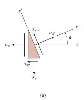
By the equations of equilibrium, we can find:

$+\nearrow \sum\,F_x\,=0$

$$\begin{align} & \sigma_{x'}\Delta\,A\,-\,(\tau_{xy}\Delta\,A\,sin\theta)cos\theta \\& -(\sigma_y\,\Delta\,A\,sin\theta)sin\theta\,-\,(\tau_{xy}\,\Delta\,A\,cos\theta)sin\theta \\& -(\sigma_x\,\Delta\,A\,cos\theta)cos\theta\,=0 \end{align}$$ $$\begin{align}\sigma_{x'}\,&=\sigma_x\,cos^2\theta\,+\,\sigma_y\,sin^2\theta\,+\tau_{xy}sin2\theta\\ & = \frac{\sigma_x+\sigma_y}{2}\,+\,\frac{\sigma_x\,-\sigma_y}{2}cos2\theta\,+\tau_{xy}sin2\theta\,\end{align} \tag{3.1}$$

$+\nwarrow \sum\,F_y\,=0$

$$\begin{align} & \tau_{x'y'}\Delta\,A\,+\,(\tau_{xy}\Delta\,A\,sin\theta)sin\theta\,-(\sigma_y\,\Delta\,A\,sin\theta)cos\theta\\&-(\tau_{xy}\,\Delta\,A\,cos\theta)cos\theta\,+\,(\sigma_x\,\Delta\,A\,cos\theta)sin\theta\,=0\end{align}$$

$\tau_{x’y’}\,=\,-\frac{1}{2}(\sigma_x-\sigma_y)sin2\theta+\tau_{xy}cos2\theta\tag{3.2}$

Differentiating $(3.1)$ in accordance with $\theta$ to make $\sigma_{x’}$ maximized,

$$\begin{align}& \frac{d\sigma_{x'}}{d\theta}\,=\, -2\sigma_x\,cos\theta\,sin\theta+2\sigma_y\,sin\theta\,cos\theta+2\tau_{xy}cos2\theta \\ & 0 = (\sigma_x\,-\,\sigma_y)sin2\theta\,-\,2\tau_{xy}cos2\theta \\ & tan2\theta\,=\,\frac{2\tau_{xy}}{\sigma_x\,-\sigma_y} \end{align}\tag{3.3}$$

If $2\theta\,=\,\alpha\,=\,tan^{-1}(\frac{2\tau_{xy}}{\sigma_x\,-\sigma_y})$, $2\theta\,=\,n\pi\,+\,\alpha\,->\,\theta\,=\,\frac{n\pi}{2}+\frac{\alpha}{2}$

If $\frac{\sigma_x\,+\,\sigma_y}{2}$is to be $\sigma_{avg}\,=\,\frac{\sigma_x\,+\,\sigma_y}{2}$, $(3.1)$ can be said to

$$\sigma_{x'}\,=\,\sigma_{avg}\,+\,\frac{\sigma_x\,-\sigma_y}{2}cos2\theta\,+\tau_{xy}sin2\theta\tag{3.4}$$

make above $\theta$ to $\theta_{x’}$, because it is about the stress along with $x’$ axis. Comparing $(3.3)$ with $(3.1)$, when the angle $\theta$ goes to $\theta_{x’}$, we can find that$\tau_{x’y’} = 0$. In other words, when the stress along the $x'$ axis is to be maximized, the stress along the $x'y'$ axis would be $0$.

For the $\theta_{x’}$, put $(3.3)$ to $(3.1)$, and the result is like below:

$\sigma_{1,2}\,=\,\frac{\sigma_x\,+\,\sigma_y}{2}\,±\sqrt{(\frac{\sigma_x\,-\,\sigma_y}{2})^2+\tau_{xy}^2}\tag{3.5}$

This is the two principal stresses.

And then, differentiating $(3.2)$ in accordance with $\theta$ to make $\tau_{x’y’}$ maximized,

$$\begin{align} & \frac{d\tau_{x'y'}}{d\theta}\,=\,-(\sigma_x\,=\,\sigma_y)cos2\theta\,-2\tau_{xy}sin2\theta \\ & 0 = \,-(\sigma_x\,=\,\sigma_y)cos2\theta\,-2\tau_{xy}sin2\theta \\ & tan2\theta\,=\,-\frac{\sigma_x\,-\sigma_y}{2\tau_{xy}} \end{align}\tag{3.6}$$

If $2\theta\,=\,\beta\,=\,tan^{-1}(-\frac{\sigma_x\,-\sigma_y}{2\tau_{xy}})$, $2\theta\,=\,n\pi\,+\,\beta\,->\,\theta\,=\,\frac{n\pi}{2}+\frac{\beta}{2}$

make above $\theta​$ to $\theta_{x’y’}​$, because it is about the stress along with $x’y’​$ axis. Comparing $(3.4)​$ with $(3.1)​$, when the angle $\theta​$ goes to $\theta_{x’y’}​$, we can find that$\sigma_{x’} = \frac{\sigma_x\,+\,\sigma_y}{2}​$. In other words, when the stress along the $x'y'​$ axis is to be maximized, the stress along the $x'​$ axis would be $\frac{\sigma_x+\sigma_y}{2}​$.

For the $\theta_{x’y’}$, put $(3.6)$ to $(3.2)$, and the result is like below:

$\tau_{1,2}\,=\,±\sqrt{(\frac{\sigma_x\,-\,\sigma_y}{2})^2\,+\,\tau_{xy}^2}\tag{3.7}$

This is the extreme of shear stresses.

Although we differentiated several formulas to find out the maximum value of $\sigma_{x’}$ and $\tau_{x’y’}$, it is still vague whether what are the direction of $\sigma_{x’}$ and $\tau_{x’y’}$. So we use the graphical method to clarify the answer for this problem.

adding the square of $(3.2)$ and $(3.4)$,

$$\begin{align}&(\sigma_{x'}-\sigma_{avg})^2\,+\tau_{x'y'}^2\,=\,R^2\\&where\,R\,=\sqrt{(\frac{\sigma_x\,-\,\sigma_y}{2})^2\,+\tau_{xy}^2}\end{align}\tag{3.8}$$

Now the representation of $(8)$ is in Fig.2 below:

Fig. 2 - Mohr's Circle for 2-D analysis

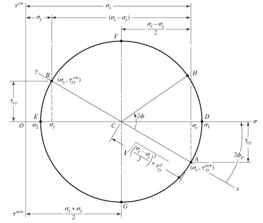
So if $\tau_{xy}$ is below the $\sigma$ axis, the shear stress acts counterclockwise for initial surface diagram in [Fig. 1], otherwise the shear stress acts clockwise. The [Fig. 2]

If you want to find the strain transformation, Replace $\sigma$ to the $\epsilon$, and $\tau$ to the $\frac{1}{2}\gamma$. Then,

$$\begin{align}&(\epsilon_{x'}-\epsilon_{avg})^2\,+{(\frac{\gamma_{x'y'}}{2})}^2\,=\,R^2\\&where\,R\,=\sqrt{(\frac{\epsilon_x\,-\,\epsilon_y}{2})^2\,+{(\frac{\gamma_{xy}}{2})}^2}\end{align}\tag{3.9}$$ 2. Stress and Strain Transformation for 2-D case: Tensor Method

Similarity transformation is used to find out the principal stress and extreme shear stress for transformed stresses.

$$\begin{align}\sigma'&\,=\,\begin{bmatrix}\sigma_{x'} & \tau_{x'y'} \\ \tau_{y'x'} & \sigma_{y'} \end{bmatrix}=\,A\,\sigma\,A^T \\ & =\begin{bmatrix}a_{xx} & a_{xy} \\ a_{yx} & a_{yy} \end{bmatrix}\begin{bmatrix}\sigma_{xx} & \tau_{xy} \\ \tau_{yx} & \sigma_{yy} \end{bmatrix}\begin{bmatrix}a_{xx} & a_{yx} \\ a_{xy} & a_{yy} \end{bmatrix} \\ &=\begin{bmatrix}cos\theta & sin\theta \\ -sin\theta & cos\theta \end{bmatrix}\begin{bmatrix}\sigma_{xx} & \tau_{xy} \\ \tau_{yx} & \sigma_{yy} \end{bmatrix}\begin{bmatrix}cos\theta & -sin\theta \\ sin\theta & cos\theta \end{bmatrix} \end{align}$$ $$\begin{align}\sigma_{x'}\,&=\sigma_x\,cos^2\theta\,+\,\sigma_y\,sin^2\theta\,+\tau_{xy}sin2\theta\\ & = \frac{\sigma_x+\sigma_y}{2}\,+\,\frac{\sigma_x\,-\sigma_y}{2}cos2\theta\,+\tau_{xy}sin2\theta\,\end{align}\tag{3.10}$$

$\tau_{x’y’}\,=\,-\frac{1}{2}(\sigma_x-\sigma_y)sin2\theta+\tau_{xy}cos2\theta\tag{3.11}$

Remained process is same to above, and for the strain we can also take the same results.

3. Conclusion

In this time, just 2-D case is driven out with both conventional method and tensor method, and we confirmed that both are to same result. Although we’ll see about whether the stress tensor method will help to derive the principal stresses out in 3-D case, we can find that the tensor representation can be strong motivation to skip the abstract graphical thinking and quick to arrive at expected result.

• References

1. R.C.Hibbeler, 10th Ed., Engineering mechanics of materials
2. Richard G. Budynas, 10th Ed., Shigley’s Mechanical Engineering Design
3. Itskov M., Tensor Algebra and Tensor Analysis for Engineers

Twitter  facebook  Google+ 

Contact

Name: * Email Address: * Message: *
* indicates a required field