2) Why tensor? (1) Dynamics of a particle in Curvilinear Motion

We’ve got seen the gradient, divergence, curl, and laplacian of a vector field or scalar function. If you are in engineering course, some of you’re going to take the engineering dynamic course.

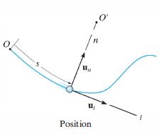
First, we would be informed about general curvilinear motion of a particle along a certain path. Let a length of moving path for a particle from the origin from time $t_i$ to $t_f$ be $s$, and the tangential path of the particle is $t$ and the normal path is $n$.

Fig. 1 - The description of movement of a particle

In calculus, you would learn that in some instantaneous moment, the particle would have a radius of curvature $\rho$ and moves for a distance of $ds$.

Fig. 2 - The concept of the radius of curvature

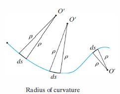
The radius of curvature is described like

$$\rho\,=\,\begin{vmatrix}\frac{d[\frac{\mathbb{v}(t)}{\begin{vmatrix}v(t) \end{vmatrix}}]}{ds} \end{vmatrix}\tag{2.1}$$

If we define $T(t)\,=\frac{r’(t)}{\begin{vmatrix}r’(t) \end{vmatrix}}\,=\,\frac{\mathbb{v(t)}}{\begin{vmatrix}\mathbb{v}(t)\end{vmatrix}}$, then

$$\rho\,=\,\begin{vmatrix}\frac{dT}{ds}\end{vmatrix}\,=\begin{vmatrix}\frac{\frac{dT}{dt}}{\frac{ds}{dt}} \end{vmatrix}\,=\,\begin{vmatrix}\frac{T'(t)}{\mathbb{v}(t)}\end{vmatrix} \tag{2.2}$$

As you can see that the motion of a particle in which condition stated before also in physics textbook, velocity has a component of direction along the path, and acceleration has components of 1) along the path and 2) perpendicular to the path. They can be expressed like

$\mathbb{v}\,=\,v\mathbb{u}_t $ Where $v\,=\,\dot{s}$

and acceleration is

$\mathbb{a}\,=\,\dot{\mathbb{v}}\,=\,\dot{v}\mathbb{u}_t\,+\,v\dot{\mathbb{u}}_t$

Fig. 3 - The motion of a particle - the relationship between u_n and u_t

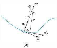
And as we can see that $\dot{\mathbb{u}}_t\,=\,\dot{\theta}\mathbb{u}_n\,=\,\frac{\dot{s}}{\rho}\mathbb{u}_n\,=\,\frac{v}{\rho}\mathbb{u}_n​$ in Fig.3, we can find that the acceleration vector $\mathbb{a}​$ would be

$\mathbb{a}\,=\,a_t\,\mathbb{u}_t\,+\,a_n\,\mathbb{u}_n$

where $a_t\,=\,\dot{v} // a_t\,ds\,=\,v\,dv$ and $a_n\,=\,\frac{v^2}{\rho}$

Graphically, in planar motion case, $\mathbb{v}\,=\,v_r\,\mathbb{u}_r\,+\,v_{\theta}\,\mathbb{u}_{\theta}$ where $v_r\,=\,\dot{r}$ and $v_{\theta}\,=\,r\dot{\theta}$, and the detail inducing process will be introduced in the post for engineering mechanics dynamics. Acceleration vector, which is the derivative of the velocity vector, is therefore $\mathbb{a}\,=\,a_r\,\mathbb{u}_r\,+\,a_{\theta}\,\mathbb{u}_{\theta}$ where $a_r\,=\,\ddot{r}-r\ddot{\theta}^2$ and $a_{\theta}\,=\,r\ddot{\theta}\,+\,2\dot{r}\dot{\theta}$.

However, we can derive the the position vector, velocity vector, and acceleration vector out much easily for 1) Cartesian(xyz-)coordinates, 2) Cylindrical(r$\theta$z-)coordinates, and 3) Spherical($\rho\phi\theta$-)coordinates. Excluding all vectors written above for cartesian coordinates(because it is just very simple), all of the stated vectors for cylindrical coordinates and spherical coordinates are like below:

-1. Cylindrical Coordinates $$\begin{align}&\hat{\mathbb{q_r}}\,=\,e_r\,=\,\frac{\frac{\partial \mathbb{r}}{\partial r}}{\begin{vmatrix}\frac{\partial \mathbb{r}}{\partial r}\end{vmatrix}}\,=\,\frac{cos\theta\,i\,+\,sin\theta\,j}{\begin{vmatrix}cos\theta\,i\,+\,sin\theta\,j\end{vmatrix}}\\&\,=\,cos\theta\,i\,+\,sin\theta\,j,\\ &\,h_r\,=\,\begin{vmatrix}\frac{\partial \mathbb{r}}{\partial r}\end{vmatrix}\,=\,1\end{align}$$ $$\begin{align}& \hat{\mathbb{q_{\theta}}}\,=\,e_{\theta}\,=\,\frac{\frac{\partial \mathbb{r}}{\partial {\theta}}}{\begin{vmatrix}\frac{\partial \mathbb{r}}{\partial {\theta}}\end{vmatrix}}\,=\,\frac{-r\,sin\theta\,i\,+\,r\,cos\theta\,j}{\begin{vmatrix}-r\,sin\theta\,i\,+\,r\,cos\theta\,j\end{vmatrix}} \\& \,=\,-sin\theta\,i\,+\,cos\theta\,j,\\&\,h_{\theta}\,=\,\begin{vmatrix}\frac{\partial \mathbb{r}}{\partial \theta}\end{vmatrix}\,=\,r\end{align}$$ $$\begin{align}& \hat{\mathbb{q_z}}\,=\,e_z\,=\,\frac{\frac{\partial \mathbb{r}}{\partial z}}{\begin{vmatrix}\frac{\partial \mathbb{r}}{\partial z}\end{vmatrix}}\,=\,\frac{k}{\begin{vmatrix}k\end{vmatrix}}\,\\&= \,k, \\&\,h_z\,=\,\begin{vmatrix}\frac{\partial \mathbb{r}}{\partial z}\end{vmatrix}\,=\,1\end{align}$$

where $x\,=\,r\,cos\theta,\,y\,=\,r\,sin\theta,\,z\,=\,z$ in cylindrical coordinates. in this time, don’t think about the $h_r\,=\,\begin{vmatrix}\frac{\partial \mathbb{r}}{\partial r}\end{vmatrix}\,=\,1$, $h_{\theta}\,=\,\begin{vmatrix}\frac{\partial \mathbb{r}}{\partial \theta}\end{vmatrix}\,=\,r$ and $h_z\,=\,\begin{vmatrix}\frac{\partial \mathbb{r}}{\partial z}\end{vmatrix}\,=\,1$ (It is same in spherical coordinates).

$$\begin{cases} \mathbb{r}\,= & re_r\,+\,ze_z \\ \mathbb{v}\,= & \frac{d\mathbb{r}}{dt}\,=\,\frac{d}{d\,t}\, (re_r\,+\,ze_z) \\ & =\,\frac{d\,r}{d\,t}e_r\,+\,r\,\frac{d\,e_r}{d\,t}\,+\frac{d\,z}{d\,t}\,e_z \\ & =\,\dot{r}\,e_r\,+\,r\,\dot{\theta}\,e_{\theta}\,+\dot{z}\,e_z \\ \mathbb{a}\,= & \frac{d\,\mathbb{v}}{d\,t} \\ & =\,\frac{d}{d\,t}\,[\dot{r}\,e_r\,+\,r\,\dot{\theta}\,e_{\theta}]\,+\,\frac{d}{d\,t}[\dot{z}\,e_z] \\ & =\,\ddot{r}\,e_r\,+\,\dot{r}\,\frac{d\,e_r}{d\,t}\,+\,\dot{r}\,\dot{\theta}\,e_{\theta}\,+\,r\,\ddot{\theta}\,e_{\theta}\,+r\,\dot{\theta}\,\cdot\,\dot{\theta}\,(-e_r)\,+\,\frac{d}{d\,t}\,(\frac{d\,z}{d\,t})e_z \\ & =\,[\ddot{r}\,-\,r({\dot{\theta}}^2)]e_r\,+\,[\dot{r}\,\ddot{\theta}\,+\,2\,\dot{r}\,\dot{\theta}]e_{\theta}\,+\,\ddot{z}\,e_z \end{cases}\tag{2.3}$$

If z-dimension is reduced, the result is same with above, the planar motion of a particle.

-2. Spherical Coordinates $$\begin{align}&\hat{\mathbb{q_{\rho}}}\,=\,e_{\rho}\,=\,\frac{\frac{\partial \mathbb{r}}{\partial \rho}}{\begin{vmatrix}\frac{\partial \mathbb{r}}{\partial \rho}\end{vmatrix}}\,=\,\frac{cos\theta\,sin\,\phi\,i\,+\,sin\theta\,sin\phi\,j\,+\,cos\phi\,k}{\begin{vmatrix}cos\theta\,sin\,\phi\,i\,+\,sin\theta\,\,sin\phi\,j\,+\,cos\phi\,k\end{vmatrix}} \\ & =\,cos\theta\,sin\,\phi\,i\,+\,sin\theta\,\,sin\phi\,j\,+\,cos\phi\,k,\\ &\,h_{\rho}\,=\,\frac{\partial \mathbb{r}}{\partial r}\,=\,1\end{align}$$ $$\begin{align}&\hat{\mathbb{q_{\theta}}}\,=\,e_{\theta}\,=\,\frac{\frac{\partial \mathbb{r}}{\partial {\theta}}}{\begin{vmatrix}\frac{\partial \mathbb{r}}{\partial {\theta}}\end{vmatrix}}\,=\,\frac{-\rho\,sin\theta\,sin\phi\,i\,+\,\rho\,cos\theta\,sin\phi\,j}{\begin{vmatrix}-\rho\,sin\theta\,sin\phi\,i\,+\,\rho\,cos\theta\,sin\phi\,j\end{vmatrix}} \\ & \,=-\,sin\theta\,i\,+\,cos\theta\,j,\, \\ & h_{\theta}\,=\,\frac{\partial \mathbb{r}}{\partial \theta}\,=\,\rho\,sin\phi\end{align}$$ $$\begin{align} & \hat{\mathbb{q_{\phi}}}\,=\,e_{\phi}\,=\,\frac{\frac{\partial \mathbb{r}}{\partial \phi}}{\begin{vmatrix}\frac{\partial \mathbb{r}}{\partial \phi}\end{vmatrix}}\,=\,\frac{\rho\,cos\theta\,cos\,\phi\,i\,+\,\rho\,sin\,\theta\,cos\phi\,j\,-\,\rho\,sin\phi\,k}{\begin{vmatrix}\rho\,cos\theta\,cos\,\phi\,i\,+\rho\,sin\,\theta\,cos\phi\,j\,-\rho\,sin\phi\,k\end{vmatrix}} \\ &\,=\,cos\theta\,cos\,\phi\,i\,+\,sin\,\theta\,cos\phi\,j\,-\,sin\phi\,k, \\ & \,h_z\,=\,\frac{\partial \mathbb{r}}{\partial z}\,=\,\rho\end{align}$$

where $x\,=\,\rho\,cos\theta\,sin\,\phi,\,y\,=\,\rho\,sin\theta\,sin\phi,\,z\,=\,\rho\,cos\phi$ in spherical coordinates.

$$\begin{cases} \mathbb{r}\,= & \rho\,e_{\rho} \\ \mathbb{v}\,= & \frac{d\,\rho}{d\,t}\,e_{\rho}\,+\,\rho\,\frac{d\,e_{\rho}}{d\,t} \\ & =\,\dot{\rho}\,e_{\rho}\,+\,\rho(\frac{\partial e_{\theta}}{\partial \theta}\,\frac{d\,\theta}{d\,t}\,+\,\frac{\partial e_{\phi}}{\partial \phi}\,\frac{d\,\phi}{d\,t}) \\ & =\,\dot{\rho}\,e_{\rho}\,+\,\rho\,\dot{\theta}\,sin\,\phi\,e_{\theta}\,+\,\rho\,\dot{\phi}\,e_{\phi} \\ \mathbb{a}\,= & \frac{d\,\mathbb{v}}{d\,t} \\ & \ddot{\rho}\,e_{\rho}\,+\,\dot{\rho}(\dot{\theta}\,sin\,\phi\,e_{\theta}\,+\,\dot{\phi}\,e_{\phi})\,+\dot{\rho}\,\dot{\theta}\,sin\,\phi\,e_{\theta} \\ & \,+\,\rho\,\ddot{\theta}\,sin\,\phi\,e_{\theta}\,+\,\rho\,\dot{\theta}\,cos\,{\phi}\,e_{\theta}\,-\,\rho\,\dot{\theta}\,sin\,\phi\,(sin\,\phi\,e_{\rho}\,+\,cos\,\phi\,e_{\phi})\,\dot{\theta} \\ &\,+\dot{\rho}\,\dot{\phi}\,e_{\phi}\,+\rho\,\ddot{\phi}\,e_{\phi}\,+\rho(\ddot{\phi}\,e_{\phi}\,+(-\dot{\phi}\,e_{\rho}\,+\,\dot{\theta}\,cos\,\phi\,e_{\theta})) \\ & =\,[\ddot{\rho}\,-\,\dot{\rho}\,{\dot{\phi}}^2\,-\,\rho\,\dot{\theta}\,sin^2\,\phi]e_{\rho} \\& \,+\,[2\,\dot{\rho}\,\dot{\theta}\,sin\,\theta\,+\,2\,\rho\,\dot{\phi}\,\dot{\theta}\,cos\,\phi\,+\,\rho\,{\dot{\theta}}^2\,sin\,\phi]e_{\theta} \\& \,+\,[\rho\,\ddot{\phi}\,+\,2\,\dot{\rho}\,\dot{\phi}\,-\,\rho\,{\dot{\theta}}^2\,sin\,\phi\,cos\,\phi]\,e_{\phi} \end{cases}\tag{2.4}$$

Believe or not, you’ll gonna study this kind of weird and, even, seems extremely hard things.

Why these kind hell of things are coming out?

To understand these things, we have to study the 1) (orthogonal) basis vector, and 2) whole differential terms of x,y,z - assume that the variables are just in $R^3$.

-3. Orthogonal basis vector

Take $q_1, q_2, q_3$ as the general orthogonal basis on $R^3$, $x, y, z$ are transformed to like:

$$\begin{align}&x\,=\,x\,(q_1,\,q_2,\,q_3),\, \\ &y\,=\,y\,(q_1,\,q_2,\,q_3)\,,\\ & z\,=\,z\,(q_1,\,q_2,\,q_3)\end{align}$$ $$\begin{align}\Leftrightarrow\,& q_1\,=\,q_1\,(x,\,y,\,z),\, \\ &q_2\,=\,q_2\,(x,\,y,\,z),\, \\ &q_3\,=\,q_3\,(x,\,y,\,z)\end{align}$$

Then a vector $\mathbb{V} $ on this coordinates basis is expressed to

$$\mathbb{V}\,=\,\hat{\mathbb{q_1}}\,V_1\,+\,\hat{\mathbb{q_2}}\,V_2\,+\hat{\mathbb{q_3}}\,V_3$$

but the position vector

$$\begin{align} \mathbb{r}&\,\neq\,\hat{\mathbb{q_1}}\,q_1\,+\,\hat{\mathbb{q_2}}\,q_2\,+\hat{\mathbb{q_3}}\,q_3, \\ & \mathbb{r}\, =\,x\,i+\,y\,j+\,z\,k\, \\ & =\,xe_1\,+\,ye_2\,+\,ze_3\end{align}$$

Position vector $\mathbb{r}​$ is often related to the cartesian coordinates. In this time, 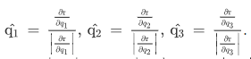Now, for the convenience of calculation, we take 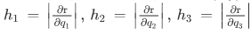so we get

-4. Whole differential terms of x,y,z $$\begin{align} &dx =\,\frac{\partial x}{\partial {q_1}}dq_1\,+\,\frac{\partial x}{\partial {q_2}}dq_2\,+\,\frac{\partial x}{\partial {q_3}}dq_3 \\ & dy=\,\frac{\partial y}{\partial {q_1}}dq_1\,+\,\frac{\partial y}{\partial {q_2}}dq_2\,+\,\frac{\partial y}{\partial {q_3}}dq_3 \\ & dz=\,\frac{\partial z}{\partial {q_1}}dq_1\,+\,\frac{\partial z}{\partial {q_2}}dq_2\,+\,\frac{\partial z}{\partial {q_3}}dq_3 \end{align}\tag{2.5}$$

and $d\mathbb{r}\,=\,dx\,i\,+\,dy\,j\,+\,dz\,k\,$

$$\begin{align}=&\,(\frac{\partial x}{\partial {q_1}}dq_1\,+\,\frac{\partial x}{\partial {q_2}}dq_2\,+\,\frac{\partial x}{\partial {q_3}}dq_3)i \\ & \,+\,(\frac{\partial y}{\partial {q_1}}dq_1\,+\,\frac{\partial y}{\partial {q_2}}dq_2\,+\,\frac{\partial y}{\partial {q_3}}dq_3)j \\ & \,+\,(\frac{\partial z}{\partial {q_1}}dq_1\,+\,\frac{\partial z}{\partial {q_2}}dq_2\,+\,\frac{\partial z}{\partial {q_3}}dq_3)k\end{align} \tag{2.6}$$

We have to define the infinitesimal length $d\mathbb{s}^2\,=\,d\mathbb{r}\,\cdot\,d\mathbb{r}\,=\,\sum_{ij}^{}\,\frac{\partial{\mathbb{r}}}{\partial{q_i}}\,\cdot\,\frac{\partial{\mathbb{r}}}{\partial{q_j}}$

$$\begin{align}=&\,g_{11}{dq_1}^2\,+\,g_{12}dq_1\,dq_2+g_{13}dq_1\,dq_3 \\ & +g_{21}dq_2\,dq_1\,+\,g_{22}{dq_2}^2\,+g_{23}dq_2\,dq_3 \\ & +g_{31}dq_3\,dq_1+\,g_{32}dq_3\,dq_2+g_{33}{dq_3}^2 \end{align}\tag{2.7}$$

Where $g_{ij}\,=\,\frac{\partial\mathbb{r}}{\partial q_i}\,\cdot\,\frac{\partial\mathbb{r}}{\partial q_j}$

Remember that we consider an “orthogonal” curvilinear coordinates. In this case, $g_{ij}\,=\,0, whose\,i ≠ j​$, so there remain the case $g_{11},\,g_{22},\,g_{33}​$. we now call the absolute value of $g_{11},\,g_{22},\,g_{33}​$ as $h_1,\,h_2,\,h_3​$.

By these ways, we can go through above proving method in -3.

• References
  1. R.C.Hibbeler, 12th Ed., Engineering Mechanics - Dynamics
  2. James Stewart, 5th Ed., Calculus
  3. Itskov M., Tensor Algebra and Tensor Analysis for Engineers

Twitter  facebook  Google+ 

Contact

Name: * Email Address: * Message: *
* indicates a required field