5) Torsinoal Load

1. Torsional Deformation of a Circular Shaft and Torsion Formula

• Torsional Deformation

Consider a shaft $AB$ subjected at $A$ and $B$ to equal and opposite torques $\mathbf{T}$ and $\mathbf{T’}$.We pass a section perpendicular to the axis of the shaft through some arbitrary point $C$ [Fig. 5.1.].

Fig. 5.1. Shaft subject to torques and a section plane at C

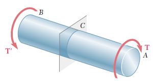
The free-body diagram of portion $BC$ of the shaft must include the elementary shearing forces $d\mathbf{F}$, which are perpendicular to the radius of the shaft. These arise from the torque that portion $AC$ exerts on $BC$ as the shaft is twisted [Fig. 5.2.a]. The conditions of equilibrium for BC require that the system of these forces be equivalent to an internal torque T, as well as equal and opposite to $\mathbf{T’}$ [Fig. 5.2.b].

Fig. 5.2. (a) Free body diagram of section BC with torque at C represented by the contributions of small elements of area carrying forces dF a radius r from the section center. (b) Free-body diagram of section BC having all the small area elements summed resulting in torque T. $$\int \rho dF = T$$

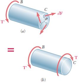
Since $ dF = \tau dA$, where $\tau$ is the shear stress on the element of area $dA$, we can write

$$\int \rho(\tau dA) = T \tag{5.1.}$$

At first, we have to study how the torsional deformation affects the form of shaft.

Fig. 5.3. Description of Torsional Deformation

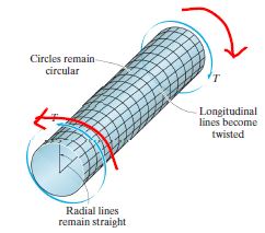
At [Fig. 5.3.], we find that when the torque is applied, the longitudinal grid lines originally marked on the shaft tend to distort into a helix, [Fig. 5.3.], that intersects the circles at equal angles. Also, all the cross sections of the shaft will remain flat—that is, they do not warp or bulge in or out—and radial lines remain straight and rotate during this deformation. Provided the angle of twist is small, then the length of the shaft and its radius will remain practically unchanged.

• Torsion Formula

Think about the one-end-fixed case, which is stated in [Fig. 5.4.]

Fig. 5.4. Description of Torsional Deformation

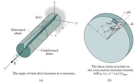
If the shaft is fixed at one end and a torque is applied to its other end, then the dark green shaded plane in [Fig. 5.4.a] will distort into a skewed form as shown. Here a radial line located on the cross section at a distance $x$ from the fixed end of the shaft will rotate through an angle $\phi(x)$. This angle is called the angle of twist. It depends on the position $x$ and will vary along the shaft as shown.

In order to understand how this distortion strains the material, we will now isolate a small disk element located at $x$ from the end of the shaft, [Fig. 5.4.b.]. Due to the deformation, the front and rear faces of the element will undergo rotation—the back face by $\phi(x)$, and the front face by $\phi(x) + d \phi$. As a result, the difference in these rotations, $d\phi$, causes the element to be subjected to a shear strain, $\gamma$ (see Fig. 5.5.).

Fig. 5.5. The Description for The Relationship Between The Shear Strain and The Angle of Twist

In [Fig. 5.4.], we get the equations that

$$\rho d \phi=dx\gamma \rightarrow \gamma=\rho \frac{d \phi}{dx} \tag{5.2.}$$

Since $dx$ and $d\phi$ are the same for all elements, then $d\phi/dx$ is constant over the cross section, and (5.1) states that the magnitude of the shear strain varies only with its radial distance r from the axis of the shaft. Since $d\phi/dx = \gamma/\rho = \gamma_{\text{max}}/c$, then

$$\gamma = \frac{\rho}{c}\gamma_{\text{max}} \tag{5.3.}$$

Since $\tau = G\gamma$, we get

$\tau=(\frac{\rho}{c})\tau_{\text{max}} \tag{5.4.}$

Combining (5.3.) and (5.4.), we get

$$\int \rho(\frac{\rho}{c} \tau_{\text{max}} dA) = T \\ \underset{\text{polar moment of inertia}}{\frac{\tau_{\text{max}}}{c}\underline{\int \rho^2 dA}} = T \tag{5.5.}$$

Replacing the $\int \rho^2 dA$ with $J$, we get

$$\tau_{\text{max}}=\frac{Tc}{J} \tag{5.6.}$$ $$\text{where}\begin{cases}\tau_{\text{max}} =& \text{the maximum shear stress in the shaft,} \\ & \text{which occurs at its outer surface} \\ T = & \text{the resultant internal torque} \\ & \text{acting at the cross section.} \\ & \text{value is determined from} \\ & \text{the method of sections and} \\ & \text{the equation of moment equilibrium} \\ & \text{applied about the shaft’s} \\ & \text{longitudinal axis} \\ J = & \text{the polar moment of inertia} \\ & \text{of the cross-sectional area} \\ c = & \text{the outer radius of the shaft} \end{cases}$$

and

$$\tau=\frac{T\rho}{J} \tag{5.7.}$$

For example, let’s find the polar moment of inertia for shaft.

$$\begin{align}J = \int_A \rho^2 dA = \int_0^c \rho^2 (2\pi \rho d\rho) \\ = 2\pi \int_0^c \rho^3 d\rho = 2\pi(\frac{1}{4})\rho^4|_0^c \\ J = \frac{\pi}{2}c^4 \end{align} \tag{5.8.}$$

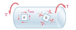
Now consider two elements a and b located on the surface of a circular shaft subjected to torsion (Fig. 3.17). Since the faces of element a are respectively parallel and perpendicular to the axis of the shaft, the only stresses on the element are the shearing stresses

$$\tau_{\text{max}}=\frac{Tc}{J}$$

On the other hand, the faces of element b, which form arbitrary angles with the axis of the shaft, are subjected to a combination of normal and shearing stresses.

Fig. 5.6. Circular shaft with stress elements at different orientations.

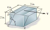
Consider the stresses and resulting forces on faces that are at $45^{\circ}$ to the axis of the shaft. The free-body diagrams of the two triangular elements are shown in [Fig. 5.7.]

Fig. 5.7. Forces on faces at 45º to shaft axis

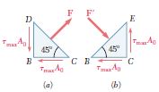
From [Fig. 5.7.a], the stresses exerted on the faces $BC$ and $BD$ are the shearing stresses $\tau_{\text{max}}=\frac{Tc}{J}$. The magnitude of the corresponding shear force is $\tau_{\text{max}}A_0$, where $A_0$ is the area of the face. Observing that the components along $DC$ of the two shear forces are equal and opposite, the force $F$ exerted on $DC$ must be perpendicular to that face and is a tensile force. Its magnitude is

$$F=2(\tau_{\text{max}}A_0)\cos45^{\circ}=\tau_{\text{max}}A_0\sqrt{2}\tag{5.9.}$$

The corresponding stress is obtained by dividing the force F by the area A of face $DC$. Observing that $A = A_0\sqrt{2}$,

$$\sigma=\frac{F}{A}=\frac{\tau_{\text{max}}A_0\sqrt{2}}{A_0\sqrt{2}}=\tau_{\text{max}}\tag{5.10.}$$

As we can see in [Fig. 5.6.], stress on ‘a’ and ‘b’ surface is the same, and therefore Torque $T$ is all the same.

2. Shear Stress Distribution.

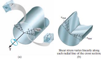
If an element of material on the cross section of the shaft or tube is isolated, then due to the complementary property of shear, equal shear stresses must also act on four of its adjacent faces, as shown in [Fig. 5.8.a.]. As a result, the internal torque T develops a linear distribution of shear stress along each radial line in the plane of the cross-sectional area, and also an associated shear-stress distribution is developed along an axial plane, [Fig. 5.8.b.]

Fig. 5.8. Description of Stress Distribution

It is interesting to note that because of this axial distribution of shear stress, shafts made of wood tend to split along the axial plane when subjected to excessive torque, [Fig. 5.9. ]

Fig. 5.9. Surficial Failure of Wood - Maximum Shear

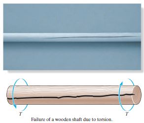
This is because wood is an anisotropic material, whereby its shear resistance parallel to its grains or fibers, directed along the axis of the shaft, is much less than its resistance perpendicular to the fibers within the plane of the cross section.

3. Angle of Twist

Recall that

$$\rho d \phi=dx\gamma \rightarrow \gamma=\rho \frac{d \phi}{dx} \tag{5.2.}$$

and

$$\gamma = \frac{\rho}{c}\gamma_{\text{max}} \tag{5.3.}$$

and last,

$$\tau_{\text{max}}=\frac{Tc}{J} \tag{5.6.}$$

Combining these formulas,

$$d\phi=\frac{T(x)}{J(x)G(x)}dx \\ \phi=\int_0^L \frac{T(x)}{J(x)G(x)}dx \tag{5.11}$$

Similarly with the axial load case,

$$\phi=\sum \frac{TL}{JG} \tag{5.12}$$

The angle of twist of one end of a shaft or tube with respect to the other end can be determined using the following procedure.

Internal Torque.

• The internal torque is found at a point on the axis of the shaft by using the method of sections and the equation of moment equilibrium, applied along the shaft’s axis.
• If the torque varies along the shaft’s length, a section should be made at the arbitrary position x along the shaft and the internal torque represented as a function of $x$, i.e., $T(x)$.
• If several constant external torques act on the shaft between its ends, the internal torque in each segment of the shaft, between any two external torques, must be determined.

Angle of Twist.

• When the circular cross-sectional area of the shaft varies along the shaft’s axis, the polar moment of inertia must be expressed as a function of its position x along the axis, $J(x)$.

• If the polar moment of inertia or the internal torque suddenly changes between the ends of the shaft, then $\phi = \int(T(x)/J(x)G(x)) dx$ or $\phi = TL/JG$ must be applied to each segment for which $J$, $G$, and $T$ are continuous or constant.

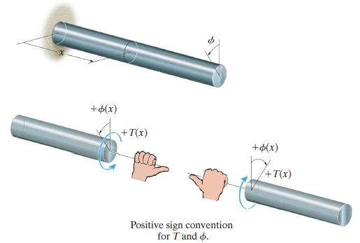
• When the internal torque in each segment is determined, be sure to use a consistent sign convention for the shaft or its segments, such as the one shown in [Fig. 5.10.] Also make sure that a consistent set of units is used when substituting numerical data into the equations.

  

Fig. 5.10. Sign Convention for The Twist Angle

4. Statically Indeterminate Torque-Loaded Members

This is also similar to the case for the statically indeterminate members with the axial load. The unknown torques in statically indeterminate shafts are determined by satisfying equilibrium, compatibility, and load–displacement requirements for the shaft.

Equilibrium.

• Draw a free-body diagram of the shaft in order to identify all the external torques that act on it. Then write the equation of moment equilibrium about the axis of the shaft.

Compatibility.

• Write the compatibility equation. Give consideration as to how the supports constrain the shaft when it is twisted.

Load–Displacement.

• Express the angles of twist in the compatibility condition in terms of the torques, using a load– displacement relation, such as $\phi = TL/JG$. • Solve the equations for the unknown reactive torques. If any of the magnitudes have a negative numerical value, it indicates that this torque acts in the opposite sense of direction to that shown on the free-body diagram.

5. Solid Noncircular Shafts, Thin-walled Tubes, Stress Concentration, and Inelastic Torsion

• Solid Noncircular Shafts

Shafts that have a noncircular cross section are not axisymmetric, and so their cross sections will bulge or warp when the shaft is twisted. Evidence of this can be seen from the way grid lines deform on a shaft having a square cross section, Fig. 5–23. Because of this deformation, the torsional analysis of noncircular shafts becomes considerably more complicated and will not be discussed in this text. *Using a mathematical analysis based on the theory of elasticity, however, the shear-stress distribution within a shaft of square cross section has been determined.*

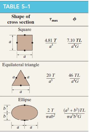
Using the theory of elasticity, Table 5–1 provides the results of the analysis for square cross sections, along with those for shafts having triangular and elliptical cross sections. In all cases, the maximum shear stress occurs at a point on the edge of the cross section that is closest to the center axis of the shaft. Also given are formulas for the angle of twist of each shaft.

Table. 5.1. Maximum Shear and Angle of Twists for Each Shape

• Thin-Walled Tubes Having Closed Cross Section

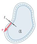
In the preceding section we saw that the determination of stresses in noncircular members generally requires the use of advanced mathematical methods. *In thin-walled hollow noncircular shafts, a good approximation of the distribution of stresses in the shaft can be obtained by a simple computation. **Consider a hollow cylindrical member of *noncircular section subjected to a torsional loading [Fig. 5.11]¹.

Fig. 5.11. Thin-walled hollow shaft subject to torsional loading.

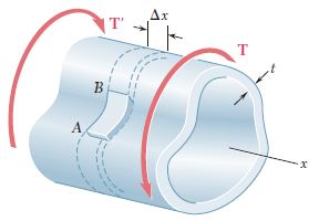
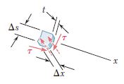
While the thickness $t$ of the wall may vary within a transverse section, it is assumed that it remains small compared to the other dimensions of the member.Now detach the colored portion of wall $AB$ bounded by two transverse planes at a distance $\Delta x$ from each other and by two longitudinal planes perpendicular to the wall. Since the portion $AB$ is in equilibrium, the sum of the forces exerted on it in the longitudinal $x$ direction must be zero (Fig. 3.48).

The only forces involved in this direction are the shearing forces $F_A$ and $F_B$ exerted on the ends of portion $AB$. Therefore,

$$\begin{matrix}\sum F_x=0; & F_A - F_B = 0 \end{matrix} \tag{5.13.}$$

Now express $F_A$ as the product of the longitudinal shearing stress $\tau_A$ on the small face at A and of the area $t_A \Delta x$ of that face:

$$F_A=\tau_A (t_A \Delta x)$$

While the shearing stress is independent of the $x$ coordinate of the point considered, it may vary across the wall. Thus, $\tau_A$ represents the average value of the stress computed across the wall. Expressing $F_B$ in a similar way and substituting for $F_A$ and $F_B$ into (5.13), write

$$\begin{matrix}\tau_A (t_A \Delta x) = \tau_B(t_B \Delta x) = 0\\\tau_A t_A = \tau_B t_B\end{matrix} \tag{5.14.}$$

Since $A$ and $B$ were chosen arbitrarily, Eq. (5.13) shows that the product $\tau t$ of the longitudinal shearing stress $\tau$ and the wall thickness $t$ is constant throughout the member. Denoting this product by $q\text{(shear flow)}$², we have

$$q = \tau t = \text{constant}\tag{5.15.}$$

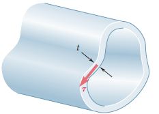
Now detach a small element from the wall portion $AB$ (Fig. 5.12.).

Fig. 5.12. Small stress element from segment

Since the outer and inner faces are part of the free surface of the hollow member, the stresses are equal to zero. the stress components indicated on the other faces by dashed arrows are also zero, while those represented by solid arrows are equal. Thus, the shearing stress at any point of a transverse section of the hollow member is parallel to the wall surface (Fig. 5.13.), and its average value computed across the wall satisfies Eq. (5.15.).

Fig. 5.13. Direction of shearing stress on cross section

At this point, an analogy can be made between the distribution of the shearing stresses $t$ in the transverse section of a thin-walled hollow shaft and the distributions of the velocities $v$ in water flowing through a closed channel of unit depth and variable width. While the velocity $v$ of the water varies from point to point on account of the variation in the width $t$ of the channel, the rate of flow, $q = vt$, remains constant throughout the channel, just as $\tau t$ in Eq. (5.15). Because of this, the product $q = \tau t$ is called the shear flow in the wall of the hollow shaft.

We will now derive a relation between the torque $T$ applied to a hollow member and the shear flow $q$ in its wall. Consider a small element of the wall section, of length $ds$ (Fig. 5.14).

Fig. 5.14. Shear force in the wall.

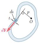
The area of the element is $dA = t ds$, and the magnitude of the shearing force $dF$ exerted on the element is

$$dF = \tau dA = \tau(t\,ds)=(\tau t)ds = q\,ds \tag{5.16.}$$

The moment $dM_O$ of this force about an arbitrary point $O$ within the cavity of the member can be obtained by multiplying $dF$ by the perpendicular distance $p$ from $O$ to the line of action of $d\mathbf{F}$.

$$dM_O = p\, dF = p(q\,ds) = q(p\,ds)\tag{5.17.}$$

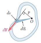
But the product $p\,ds$ is equal to twice the area $d\mathfrak{A}$ of the colored triangle in [Fig. 5.15.].

Fig. 5.15. Infinitesimal area used in finding the resultant torque.

Thus,

$$dM_O = q(2d\mathfrak{A}) \tag{5.18.}$$

Since the integral around the wall section of the left-hand member of Eq. (5.18.) represents the sum of the moments of all the elementary shearing forces exerted on the wall section and this sum is equal to the torque T applied to the hollow member,

$$T=\oint dM_O = \oint q(2d\mathfrak{A})$$

The shear flow $q$ being a constant, write

$$T = 2q\mathfrak{A}\tag{5.19.}$$

where $\mathfrak{A}$ is the area bounded by the center line of the wall cross section (Fig. 5.16.).

Fig. 5.16. Area for shear flow.

The shearing stress $\tau$ at any given point of the wall can be expressed in terms of the torque $T$ if $q$ is substituted from Eq. (5.15) into Eq. (5.19). Solving for $\tau$:

$$\tau = \frac{T}{2t\mathfrak{A}} \tag{5.20.}$$

where t is the wall thickness at the point considered and A the area bounded by the center line. Recall that t represents the average value of the shearing stress across the wall. However, for elastic deformations, the distribution of stresses across the wall can be assumed to be uniform, and thus Eq. (5.20.) yields the actual shearing stress at a given point of the wall.

The angle of twist of a thin-walled hollow shaft can be obtained also by using the method of energy. Assuming an elastic deformation, it is shown that the angle of twist of a thin-walled shaft of length $L$ and modulus of rigidity $G$ is

$$\phi = \frac{TL}{4\mathfrak{A}^2G}\oint\frac{ds}{t}\tag{5.21.}$$

where the integral is computed along the center line of the wall section.

• Stress Concentration

The torsion formula, $\tau_{\text{max}} = Tc/J$, cannot be applied to regions of a shaft having a sudden change in the cross section, because the shear-stress and shear-strain distributions in the shaft become complex. Results can be obtained, however, by using experimental methods or possibly by a mathematical analysis based on the theory of elasticity.

Fig. 5.17. K value for the r/d ratio

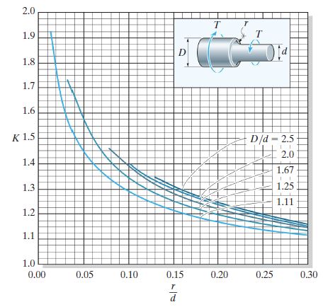
Similar to the case of axial load, $K = \frac{\tau_{\text{max}}}{\tau{\text{_avg}}}$. Then,

$$\tau_{\text{max}} = K\frac{Tc}{J}\tag{5.22.}$$

• Plastic Deformations in Circular Shafts Made of an Elastoplastic Material

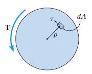
If the torsional loadings applied to the shaft are excessive, then the material may yield, and, consequently, a “plastic analysis” must be used to determine the shear-stress distribution and the angle of twist. the shear strains that develop in a circular shaft will vary linearly, from zero at the center of the shaft to a maximum at its outer boundary. This is referred to “idealized case of a solid circular shaft made of an elastoplastic material”. Since the shear stress $\tau$ acting on an element of area $dA$, [Fig. 5.18.] produces a force of $dF = \tau dA$, then the torque about the axis of the shaft is $dT = \rho dF = \rho(\tau dA)$.

Fig. 5.18. Diagram To Define The Stress Distribution on The Elasto-Plastic Shaft

For the entire shaft we require

$$T = \int_A \rho \tau dA \tag{5.23.}$$

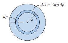
If the area $dA$ over which $\tau$ acts is defined as a differential ring having an area of $dA = 2\pi \rho d\rho$, Fig. 5.19, then the above equation can be written as

Fig. 5.19. Diagram For the Formula (5.22.) $$T = 2\pi \int_0^c \tau \rho^2 d\rho$$

We will now apply this equation to a shaft that is subjected to two types of torque.

• Elasto-Plastic Torque.

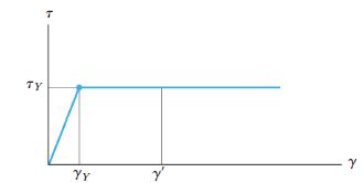
Let us consider the material in the shaft to exhibit an elastic perfectly plastic behavior, as shown in [Fig. 5.20.].

Fig. 5.20 Stress-Strain Diagram for the Elasto-Plastic

Recall that

$$\tau_{\text{max}}=\frac{Tc}{J} \tag{5.6.}$$

Similar to the case of axial load, the shear stress increases linearly in radial direction until the shear reaches the yielding shear stress.

Fig. 5.21. Shear Distribution for Elasto-plastic Shaft a) Elastic b) Impending Yield c) Partially Yielded d) Fully Yielded

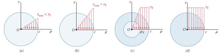
In [Fig 5.21. b)], which means that the shear arrives at the yielding stress. In this stage, Torque is to be stagnated in

$$T_Y = \frac{J}{c}\tau_Y \tag{5.24.}$$

For a solid circular shaft, $\frac{J}{c} = \frac{\pi c^3}{2}$, so we have

$$T_Y = \frac{\pi c^3}{2}\tau_Y \tag{5.25.}$$

As $T$ is increased, the plastic region is propagated, which leads to the increase of slope - No, it doesn’t mean that the shear modulus increased. The shear stress reached at its elastic limitation. - in the stress-strain diagram. As in [Fig. 5.21. c)], the shear stress increases to the elastic limit within the elastic core of radius $\rho_Y$, and by this the shear stress is expressed as

$$\tau=\frac{\tau_Y}{\rho_Y}\rho \tag{5.26.}$$

As (5.26.) is applied to the (5.23.), we get the torque as

$$\begin{align} T= & \int_0^{\rho_Y}\rho \frac{\tau_Y}{\rho_Y}\rho (2\pi \rho d\rho) + \int_{\rho_Y}^c \rho \tau_Y (2\pi\rho)d\rho \\ & = \frac{\pi}{2}\tau_Y \rho_Y^3 + \frac{2}{3}\pi(c^3 - \rho_Y^3) \\ & = \frac{2}{3}\pi\tau_Yc^3(1-\frac{1}{4}\frac{\rho_Y^3}{c^3})\end{align}\tag{5.27.}$$

As seeing through the perspective of the yielding torque, we get another formula:

$$T = \frac{4}{3}T_Y(1-\frac{1}{4} \frac{\rho_Y^3}{c^3}) \tag{5.28.}$$

If the plastic deformation is completed, which means that $\rho_Y = 0$, we get the plastic torque $T_p$ as

$$T_p = \frac{4}{3}T_Y \tag{5.29.}$$

Note that (5.28.) is valid only for a solid circular shaft made of an elastoplastic material. Since the distribution of strain across the section remains linear after the onset of yield, following equations

$$L \gamma = \rho \phi \tag{5.30.}$$ $$L \gamma_{max} = c \phi \tag{5.31.}$$

remains valid and can be used to express the radius $\rho_Y$ of the elastic core in terms of the angle of twist $\phi$. If $\phi$ is large enough to cause a plastic deformation, the radius $\rho_Y$ of the elastic core is obtained by making $\gamma$ equal to the yield strain $\gamma_Y$ in (5.30.) and solving for the corresponding value $\rho_Y$ of the distance $\rho$.

$$\rho_Y = \frac{L \gamma_Y}{\phi} \tag{5.32.}$$ $$c = \frac{L \gamma_Y}{\phi_Y} \tag{5.33.}$$

where $\phi_Y$: the angle of twist at the onset of yield (In other words, the verge of yielding deformation). Dividing (5.32.) by (5.33.), we can get

$$\frac{\rho_Y}{c} = \frac{\phi_Y}{\phi} \tag{5.34.}$$

If we carry the expression obtained for $\frac{\rho_Y}{c}$ into (5.28.), the torque $T$ as a function of the angle of twist $\phi$ is

$$T=\frac{4}{3}T_Y(1-\frac{1}{4}\frac{\phi_Y^3}{\phi^3}) \tag{5.35.}$$

To drill into the transition process in the elastoplastic material, let us see a figure.

Fig. 5.22 Load-Displacement Relation for elastoplastic material.

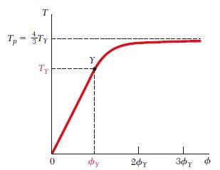
So, the overall formula of elastoplastic torque according to the angle of twist is expressed by

$$T = \begin{cases}\frac{T_Y}{\phi_Y}\phi & \phi\leq \phi_Y \\ \frac{4}{3}T_Y(1-\frac{1}{4}\frac{\phi_Y^3}{\phi^3}) & \phi > \phi_Y \end{cases} \tag{5.36.}$$

Note that (5.34.) can be used only for values of $\phi$ larger than $\phi_Y$. For $\phi<\phi_Y$, the relation between $T$ and $\phi$ is linear and given by (5.12.). Combining both equations, the plot of $T$ against $\phi$ is as represented in [Fig. 5.22.] As $\phi$ increases indefinitely, $T$ approaches the limiting value $T_p=\frac{4}{3}T_Y$ corresponding to the case of a fully developed plastic zone [Fig. 5.21.d)] While the value $T_p$ cannot actually be reached, (5.35.) indicates that it is rapidly approached as f increases. For $\phi = 2 \phi_Y$, $T$ is within about 3% of $T_p$, and for $\phi = 3 \phi_Y$, it is within about 1%.

Since the plot of $T$ against $\phi$ for an idealized elastoplastic material [Fig. 5.22.] differs greatly from the shearing-stress-strain diagram [Fig. 5.20], it is clear that the shearing-stress-strain diagram of an actual material cannot be obtained directly from a torsion test carried out on a solid circular rod made of that material. However, a fairly accurate diagram can be obtained from a torsion test if a portion of the specimen consists of a thin circular tube.³ Indeed, the shearing stress will have a constant value $\tau$ in that portion. Thus, (5.1.) reduces to

$$T=\rho A \tau$$

where $\rho$ is the average radius of the tube and $A$ is its cross-sectional area. The shearing stress is proportional to the torque, and $\tau$ easily can be computed from the corresponding values of $T$. The corresponding shearing strain $\gamma$ can be obtained from (5.31.) and from the values of $\phi$ and $L$ measured on the tubular portion of the specimen.

6. Residual Stresses in Circular Shafts

Fig. 5.23. Nonlinear shearing-stress-strain diagram.

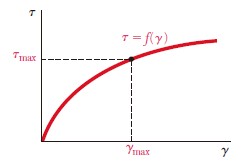
we saw that a plastic region will develop in a shaft subjected to a large enough torque, and that the shearing stress $\tau$ at any given point in the plastic region may be obtained from the shearing-stress- strain diagram of [Fig. 5.23.] If the torque is removed, the resulting reduction of stress and strain at the point considered will take place along a straight line [Fig. 5.24.].

Fig. 5.24. Shear stress-strain diagram for loading past yield, followed by unloading until compressive yield occurs.

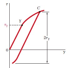
As you will see further in this section, the final value of the stress will not, in general, be zero. There will be a residual stress at most points, and that stress may be either positive or negative. We note that, as was the case for the normal stress, the shearing stress will keep decreasing until it has reached a value equal to its maximum value at $C$ minus twice the yield strength of the material.

Consider [Fig. 5.20] again to see more things. Similar to the case of the axial load, there occurs the plastic angle of twist deformation. Assuming that the relationship between t and g at any point of the shaft remains linear as long as the stress does not decrease by more than $2\tau_Y$, we can use (5.11.) to obtain the angle through which the shaft untwists as the torque decreases back to zero.As a result, the unloading of the shaft is represented by a straight line on the T-f diagram [Fig. 5.25.].

Fig. 5.25. Torque-angle of twist response for loading past yield, followed by unloading.

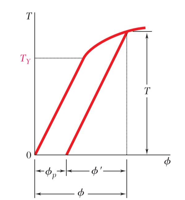
Note that the angle of twist does not return to zero after the torque has been removed. Indeed, the loading and unloading of the shaft result in a permanent deformation characterized by

$$\phi_p\,=\,\phi - \phi' \tag{5.37.}$$

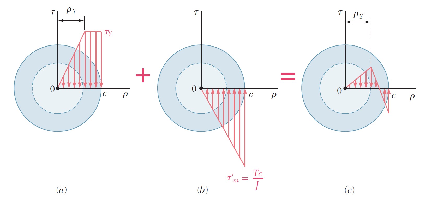
where $\phi$ corresponds to the loading phase and can be obtained from T by solving (5.36.) with $\phi’$ corresponding to the unloading phase obtained from (5.12.). [Fig. 5.26] represents overall stress distribution of elastoplastic material due to residual stress for unloading.

Fig. 5.26. Torque-angle of twist response for loading past yield, followed by unloading.

7. Design of Transmission Shafts

The principal specifications to be met in the design of a transmission shaft are the power to be transmitted and the speed of rotation of the shaft. The role of the designer is to select the material and the dimensions of the cross section of the shaft so that the maximum shearing stress allowable will not be exceeded when the shaft is transmitting the required power at the specified speed.

To determine the torque exerted on the shaft, the power $P$ associated with the rotation of a rigid body subjected to a torque $T$ is

$$P = T \omega \tag{5.38.}$$

Where $\omega$ is the angular velocity of the body in radians per second (rad/s). But $\omega = 2\pi f$, where $f$ is the frequency of the rotation, (i.e., the number of revolutions per second). The unit of frequency is $1 s^{-1}$ and is called a hertz (Hz). Substituting for v into (5.38.),

$$P = 2\pi f T \tag{5.39.}$$

When SI units are used with $f$ expressed in Hz and $T$ in N·m, the power will be in N·m/s—that is, in watts (W). Solving (5.39.) for T, the torque exerted on a shaft transmitting the power $P$ at a frequency of rotation $f$ is

$$T = \frac{P}{2 \pi f} \tag{5.40.}$$

After determining the torque $T$ to be applied to the shaft and selecting the material to be used, the designer carries the values of $T$ and the maximum allowable stress into (5.6.).

$$\frac{J}{c} = \frac{T}{\tau_{max}} \tag{5.41.}$$

This also provides the minimum allowable parameter $\frac{J}{c}$. When SI units are used, $T$ is expressed in N·m, $\tau_{max}$ in Pa (or N/m2), and $\frac{J}{c}$ in m^3. For a solid circular shaft, $J = \frac{1}{2}\pi c^4$, and $\frac{J}{c} = \frac{1}{2}\pi c^3$; substituting this value for $\frac{J}{c}$ into (5.41.) and solving for $c$ yields the minimum allowable value for the radius of the shaft. For a hollow circular shaft, the critical parameter is $\frac{J}{c_2}$, where $c_2$ is the outer radius of the shaft; the value of this parameter may be computed from Eq. (5.7.) to determine whether a given cross section will be acceptable.

For utmost long time, we’ve seen about the torsion. In most case we can find the similarity in angle of twist, statically indeterminate shafts, stress concentration, residual stress and plastic deformation of shaft. seeing from similarities to specific differences, one can will have been getting used to find the axial load and torsional load out for a given situation by the end of this lecture.

References

• R.C. Hibbeler, “Mechanics of materials”, Pearson, 10th ed., ch.5
• Ferdinand P. Beer, Mechanics of Materials, 5th ed., ch.3

1. The wall of the member must enclose a single cavity and must not be slit open. In other words, the member should be topologically equivalent to a hollow circular shaft. ↩

2. The terminology “flow” is used since q is analogous to water flowing through a channel of rectangular cross section having a constant depth and variable width. ↩

3. In order to minimize the possibility of failure by buckling, the specimen should be made so that the length of the tubular portion is no longer than its diameter. ↩

Twitter  facebook  Google+ 

Contact

Name: * Email Address: * Message: *
* indicates a required field